AI Applications in the fields of Multimedia, Computer Vision and Robotics: Scale-invariant feature transform

Article From Wikipedia

For any object in an image, there are many 'features' which are interesting points on the object, that can be extracted to provide a "feature" description of the object. This description extracted from a training image can then be used to identify the object when attempting to locate the object in a test image containing many other objects. It is important that the set of features extracted from the training image is robust to changes in image scale, noise, illumination and local geometric distortion, for performing reliable recognition. Lowe's patented method can robustly identify objects even among clutter and under partial occlusion because his SIFT feature descriptor is invariant to scale, orientation, affine distortion and partially invariant to illumination changes. This section presents Lowe's object recognition method in a nutshell and mentions a few competing techniques available for object recognition under clutter and partial occlusion.

David Lowe's method

SIFT keypoints of objects are first extracted from a set of reference images and stored in a database. An object is recognized in a new image by individually comparing each feature from the new image to this database and finding candidate matching features based on Euclidean distance of their feature vectors. From the full set of matches, subsets of keypoints that agree on the object and its location, scale, and orientation in the new image are identified to filter out good matches. The determination of consistent clusters is performed rapidly by using an efficient hash table implementation of the generalized Hough transform. Each cluster of 3 or more features that agree on an object and its pose is then subject to further detailed model verification and subsequently outliers are discarded. Finally the probability that a particular set of features indicates the presence of an object is computed, given the accuracy of fit and number of probable false matches. Object matches that pass all these tests can be identified as correct with high confidence.

Key stages

Scale-invariant feature detection

Lowe's method for image feature generation called the Scale Invariant Feature Transform (SIFT) transforms an image into a large collection of feature vectors, each of which is invariant to image translation, scaling, and rotation, partially invariant to illumination changes and robust to local geometric distortion. These features share similar properties with neurons in inferior temporal cortex that are used for object recognition in primate vision. Key locations are defined as maxima and minima of the result of difference of Gaussians function applied in scale-space to a series of smoothed and resampled images. Low contrast candidate points and edge response points along an edge are discarded. Dominant orientations are assigned to localized keypoints. These steps ensure that the keypoints are more stable for matching and recognition. SIFT descriptors robust to local affine distortion are then obtained by considering pixels around a radius of the key location, blurring and resampling of local image orientation planes.

Feature matching and indexing

Indexing is the problem of storing SIFT keys and identifying matching keys from the new image. Lowe used a modification of the k-d tree algorithm called the Best-bin-first search method that can identify the nearest neighbors with high probability using only a limited amount of computation. The BBF algorithm uses a modified search ordering for the k-d tree algorithm so that bins in feature space are searched in the order of their closest distance from the query location. This search order requires the use of a heap (data structure) based priority queue for efficient determination of the search order. The best candidate match for each keypoint is found by identifying its nearest neighbor in the database of keypoints from training images. The nearest neighbors are defined as the keypoints with minimum Euclidean distance from the given descriptor vector. The probability that a match is correct can be determined by taking the ratio of distance from the closest neighbor to the distance of the second closest.

Lowe rejected all matches in which the distance ratio is greater than 0.8, which eliminates 90% of the false matches while discarding less than 5% of the correct matches. To further improve the efficiency of the best-bin-first algorithm search was cut off after checking the first 200 nearest neighbor candidates. For a database of 100,000 keypoints, this provides a speedup over exact nearest neighbor search by about 2 orders of magnitude yet results in less than a 5% loss in the number of correct matches.

Cluster identification by Hough transform voting

Hough Transform is used to cluster reliable model hypotheses to search for keys that agree upon a particular model pose. Hough transform identifies clusters of features with a consistent interpretation by using each feature to vote for all object poses that are consistent with the feature. When clusters of features are found to vote for the same pose of an object, the probability of the interpretation being correct is much higher than for any single feature. An entry in a hash table is created predicting the model location, orientation, and scale from the match hypothesis.The hash table is searched to identify all clusters of at least 3 entries in a bin, and the bins are sorted into decreasing order of size.

Each of the SIFT keypoints specifies 2D location, scale, and orientation, and each matched keypoint in the database has a record of the keypoint’s parameters relative to the training image in which it was found. The similarity transform implied by these 4 parameters is only an approximation to the full 6 degree-of-freedom pose space for a 3D object and also does not account for any non-rigid deformations. Therefore, Lowe used broad bin sizes of 30 degrees for orientation, a factor of 2 for scale, and 0.25 times the maximum projected training image dimension (using the predicted scale) for location. The SIFT key samples generated at the larger scale are given twice the weight of those at the smaller scale. This means that the larger scale is in effect able to filter the most likely neighbours for checking at the smaller scale. This also improves recognition performance by giving more weight to the least-noisy scale. To avoid the problem of boundary effects in bin assignment, each keypoint match votes for the 2 closest bins in each dimension, giving a total of 16 entries for each hypothesis and further broadening the pose range.

[edit] Model verification by linear least squares

Each identified cluster is then subject to a verification procedure in which a linear least squares solution is performed for the parameters of the affine transformation relating the model to the image. The affine transformation of a model point [x y]^T to an image point [u v]^T can be written as below

$\begin{bmatrix} u \\ v \end{bmatrix} = \begin{bmatrix} m1 & m2 \\ m3 & m4 \end{bmatrix} \begin{bmatrix} x \\ y \end{bmatrix} + \begin{bmatrix} tx \\ ty \end{bmatrix}$

where the model translation is [tx ty]^T and the affine rotation, scale, and stretch are represented by the parameters m1, m2, m3 and m4. To solve for the transformation parameters the equation above can be rewritten to gather the unknowns into a column vector.

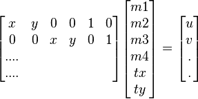
$\begin{bmatrix} x & y & 0 & 0 & 1 & 0 \\ 0 & 0 & x & y & 0 & 1 \\ ....\\ ....\end{bmatrix} \begin{bmatrix}m1 \\ m2 \\ m3 \\ m4 \\ tx \\ ty \end{bmatrix} = \begin{bmatrix} u \\ v \\ . \\ . \end{bmatrix}$

This equation shows a single match, but any number of further matches can be added, with each match contributing two more rows to the first and last matrix. At least 3 matches are needed to provide a solution. We can write this linear system as

$A\hat{\mathbf{x}} \approx \mathbf{b},$

where A is a known m-by-n matrix (usually with m > n), x is an unknown n-dimensional parameter vector, and b is a known m-dimensional measurement vector.

Therefore the minimizing vector $\hat{\mathbf{x}}$ is a solution of the normal equation

$A^T \! A \hat{\mathbf{x}} = A^T \mathbf{b}.$

The solution of the system of linear equations is given in terms of the matrix (A^TA) ^{− 1}A^T , called the pseudoinverse of A, by

$\hat{\mathbf{x}} = (A^T\!A)^{-1} A^T \mathbf{b}.$

which minimizes the sum of the squares of the distances from the projected model locations to the corresponding image locations.

Outlier detection

Outliers can now be removed by checking for agreement between each image feature and the model, given the parameter solution. Given the linear least squares solution, each match is required to agree within half the error range that was used for the parameters in the Hough transform bins. As outliers are discarded, the linear least squares solution is re-solved with the remaining points, and the process iterated. If fewer than 3 points remain after discarding outliers, then the match is rejected. In addition, a top-down matching phase is used to add any further matches that agree with the projected model position, which may have been missed from the Hough transform bin due to the similarity transform approximation or other errors.

The final decision to accept or reject a model hypothesis is based on a detailed probabilistic model. This method first computes the expected number of false matches to the model pose, given the projected size of the model, the number of features within the region, and the accuracy of the fit. A Bayesian probability analysis then gives the probability that the object is present based on the actual number of matching features found. A model is accepted if the final probability for a correct interpretation is greater than 0.98. Lowe's SIFT based object recognition gives excellent results except under wide illumination variations and under non-rigid transformations.

Competing methods for scale invariant object recognition under clutter / partial occlusion

RIFT is a rotation-invariant generalization of SIFT. The RIFT descriptor is constructed using circular normalized patches divided into concentric rings of equal width and within each ring a gradient orientation histogram is computed. To maintain rotation invariance, the orientation is measured at each point relative to the direction pointing outward from the center.

G-RIF : Generalized Robust Invariant Feature is a general context descriptor which encodes edge orientation, edge density and hue information in a unified form combining perceptual information with spatial encoding. The object recognition scheme uses neighbouring context based voting to estimate object models.

"SURF : Speeded Up Robust Features" is a high-performance scale and rotation-invariant interest point detector / descriptor claimed to approximate or even outperform previously proposed schemes with respect to repeatability, distinctiveness, and robustness. SURF relies on integral images for image convolutions to reduce computation time, builds on the strengths of the leading existing detectors and descriptors (using a fast Hessian matrix-based measure for the detector and a distribution-based descriptor). It describes a distribution of Haar wavelet responses within the interest point neighbourhood. Integral images are used for speed and only 64 dimensions are used reducing the time for feature computation and matching. The indexing step is based on the sign of the Laplacian,which increases the matching speed and the robustness of the descriptor.

PCA-SIFT and GLOH are variants of SIFT. PCA-SIFT descriptor is a vector of image gradients in x and y direction computed within the support region. The gradient region is sampled at 39x39 locations, therefore the vector is of dimension 3042. The dimension is reduced to 36 with PCA. Gradient location-orientation histogram (GLOH) is an extension of the SIFT descriptor designed to increase its robustness and distinctiveness. The SIFT descriptor is computed for a log-polar location grid with three bins in radial direction (the radius set to 6, 11, and 15) and 8 in angular direction, which results in 17 location bins. The central bin is not divided in angular directions. The gradient orientations are quantized in 16 bins resulting in 272 bin histogram. The size of this descriptor is reduced with PCA. The covariance matrix for PCA is estimated on image patches collected from various images. The 128 largest eigenvectors are used for description.

Wagner et al. developed two object recognition algorithms especially designed with the limitations of current mobile phones in mind. In contrast to the classic SIFT approach Wagner et al. use the FAST corner detector for feature detection. The algorithm also distinguishes between the off-line preparation phase where features are created at different scale levels and the on-line phase where features are only created at the current fixed scale level of the phone's camera image. In addition, features are created from a fixed patch size of 15x15 pixels and form a SIFT descriptor with only 36 dimensions. The approach has been further extended by integrating a Scalable Vocabulary Tree in the recognition pipeline. This allows the efficient recognition of a larger number of objects on mobile phones. The approach is mainly restricted by the amount of available RAM.

Features

The detection and description of local image features can help in object recognition. The SIFT features are local and based on the appearance of the object at particular interest points, and are invariant to image scale and rotation. They are also robust to changes in illumination, noise, and minor changes in viewpoint. In addition to these properties, they are highly distinctive, relatively easy to extract, allow for correct object identification with low probability of mismatch and are easy to match against a (large) database of local features. Object description by set of SIFT features is also robust to partial occlusion; as few as 3 SIFT features from an object are enough to compute its location and pose. Recognition can be performed in close-to-real time, at least for small databases and on modern computer hardware.

Algorithm

Scale-space extrema detection

This is the stage where the interest points, which are called keypoints in the SIFT framework, are detected. For this, the image is convolved with Gaussian filters at different scales, and then the difference of successive Gaussian-blurred images are taken. Keypoints are then taken as maxima/minima of the Difference of Gaussians (DoG) that occur at multiple scales. Specifically, a DoG image $D \left( x, y, \sigma \right)$ is given by

$D \left( x, y, \sigma \right) = L \left( x, y, k_i\sigma \right) - L \left( x, y, k_j\sigma \right)$ ,

where $L \left( x, y, k\sigma \right)$ is the convolution of the original image $I \left( x, y \right)$ with the Gaussian blur $G \left( x, y, k\sigma \right)$ at scale kσ, i.e.,

$L \left( x, y, k\sigma \right) = G \left( x, y, k\sigma \right) * I \left( x, y \right)$

Hence a DoG image between scales k_iσ and k_jσ is just the difference of the Gaussian-blurred images at scales k_iσ and k_jσ. For scale-space extrema detection in the SIFT algorithm, the image is first convolved with Gaussian-blurs at different scales. The convolved images are grouped by octave (an octave corresponds to doubling the value of σ), and the value of k_i is selected so that we obtain a fixed number of convolved images per octave. Then the Difference-of-Gaussian images are taken from adjacent Gaussian-blurred images per octave.

Once DoG images have been obtained, keypoints are identified as local minima/maxima of the DoG images across scales. This is done by comparing each pixel in the DoG images to its eight neighbors at the same scale and nine corresponding neighboring pixels in each of the neighboring scales. If the pixel value is the maximum or minimum among all compared pixels, it is selected as a candidate keypoint.

This keypoint detection step is a variation of one of the blob detection methods developed by Lindeberg by detecting scale-space extrema of the scale normalized Laplacian,that is detecting points that are local extrema with respect to both space and scale, in the discrete case by comparisons with the nearest 26 neighbours in a discretized scale-space volume. The difference of Gaussians operator can be seen as an approximation to the Laplacian, here expressed in a pyramid setting.

Keypoint localization

After scale space extrema are detected (their location being shown in the uppermost image) the SIFT algorithm discards low contrast keypoints (remaining points are shown in the middle image) and then filters out those located on edges. Resulting set of keypoints is shown on last image.

Scale-space extrema detection produces too many keypoint candidates, some of which are unstable. The next step in the algorithm is to perform a detailed fit to the nearby data for accurate location, scale, and ratio of principal curvatures. This information allows points to be rejected that have low contrast (and are therefore sensitive to noise) or are poorly localized along an edge.

Interpolation of nearby data for accurate position

First, for each candidate keypoint, interpolation of nearby data is used to accurately determine its position. The initial approach was to just locate each keypoint at the location and scale of the candidate keypoint.The new approach calculates the interpolated location of the extremum, which substantially improves matching and stability.The interpolation is done using the quadratic Taylor expansion of the Difference-of-Gaussian scale-space function, $D \left( x, y, \sigma \right)$ with the candidate keypoint as the origin. This Taylor expansion is given by:

$D(\textbf{x}) = D + \frac{\partial D^T}{\partial \textbf{x}}\textbf{x} + \frac{1}{2}\textbf{x}^T \frac{\partial^2 D}{\partial \textbf{x}^2} \textbf{x}$

where D and its derivatives are evaluated at the candidate keypoint and $\textbf{x} = \left( x, y, \sigma \right)$ is the offset from this point. The location of the extremum, $\hat{\textbf{x}}$ , is determined by taking the derivative of this function with respect to $\textbf{x}$ and setting it to zero. If the offset $\hat{\textbf{x}}$ is larger than 0.5 in any dimension, then that's an indication that the extremum lies closer to another candidate keypoint. In this case, the candidate keypoint is changed and the interpolation performed instead about that point. Otherwise the offset is added to its candidate keypoint to get the interpolated estimate for the location of the extremum. A similar subpixel determation of the locations of scale-space extrema is performed in the real-time implementation based on hybrid pyramids developed by Lindeberg and his co-workers

Discarding low-contrast keypoints

To discard the keypoints with low contrast, the value of the second-order Taylor expansion $D(\textbf{x})$ is computed at the offset $\hat{\textbf{x}}$ . If this value is less than 0.03, the candidate keypoint is discarded. Otherwise it is kept, with final location $\textbf{y} + \hat{\textbf{x}}$ and scale σ, where $\textbf{y}$ is the original location of the keypoint at scale σ.

Eliminating edge responses

The DoG function will have strong responses along edges, even if the candidate keypoint is unstable to small amounts of noise. Therefore, in order to increase stability, we need to eliminate the keypoints that have poorly determined locations but have high edge responses.

For poorly defined peaks in the DoG function, the principal curvature across the edge would be much larger than the principal curvature along it. Finding these principal curvatures amounts to solving for the eigenvalues of the second-order Hessian matrix, H:

$\textbf{H} = \begin{bmatrix} D_{xx} & D_{xy} \\ D_{xy} & D_{yy} \end{bmatrix}$

The eigenvalues of H are proportional to the principal curvatures of D. It turns out that the ratio of the two eigenvalues, say α is the larger one, and β the smaller one, with ratio r = α / β, is sufficient for SIFT's purposes. The trace of H, i.e., D_xx + D_yy, gives us the sum of the two eigenvalues, while its determinant, i.e., 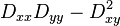$D_{xx} D_{yy} - D_{xy}^2$ , yields the product. The ratio $\text{R} = \operatorname{Tr} \left( \textbf{H} \right)^2/\operatorname{Det} \left( \textbf{H} \right)$ can be shown to be equal to $\left( r+1 \right)^2/r$ , which depends only on the ratio of the eigenvalues rather than their individual values. R is minimum when the eigenvalues are equal to each other. Therefore the higher the absolute difference between the two eigenvalues, which is equivalent to a higher absolute difference between the two principal curvatures of D, the higher the value of R. It follows that, for some threshold eigenvalue ratio r_th, if R for a candidate keypoint is larger than $\left( r_{\text{th}} + 1 \right)^2/r_{\text{th}}$ , that keypoint is poorly localized and hence rejected. The new approach uses r_th = 10.

This processing step for suppressing responses at edges is a transfer of a corresponding approach in the Harris operator for corner detection. The difference is that the measure for thresholding is computed from the Hessian matrix instead of a second-moment matrix (see structure tensor).

Orientation assignment

In this step, each keypoint is assigned one or more orientations based on local image gradient directions. This is the key step in achieving invariance to rotation as the keypoint descriptor can be represented relative to this orientation and therefore achieve invariance to image rotation.

First, the Gaussian-smoothed image $L \left( x, y, \sigma \right)$ at the keypoint's scale σ is taken so that all computations are performed in a scale-invariant manner. For an image sample $L \left( x, y \right)$ at scale σ, the gradient magnitude, $m \left( x, y \right)$ , and orientation, $\theta \left( x, y \right)$ , are precomputed using pixel differences:

$m \left( x, y \right) = \sqrt{\left( L \left( x+1, y \right) - L \left( x-1, y \right) \right)^2 + \left( L \left( x, y+1 \right) - L \left( x, y-1 \right) \right)^2}$

$\theta \left( x, y \right) = \tan^{-1}\left(\frac{L \left( x, y+1 \right) - L \left( x, y-1 \right)}{L \left( x+1, y \right) - L \left( x-1, y \right)} \right)$

The magnitude and direction calculations for the gradient are done for every pixel in a neighboring region around the keypoint in the Gaussian-blurred image L. An orientation histogram with 36 bins is formed, with each bin covering 10 degrees. Each sample in the neighboring window added to a histogram bin is weighted by its gradient magnitude and by a Gaussian-weighted circular window with a σ that is 1.5 times that of the scale of the keypoint. The peaks in this histogram correspond to dominant orientations. Once the histogram is filled, the orientations corresponding to the highest peak and local peaks that are within 80% of the highest peaks are assigned to the keypoint. In the case of multiple orientations being assigned, an additional keypoint is created having the same location and scale as the original keypoint for each additional orientation.

Keypoint descriptor

Previous steps found keypoint locations at particular scales and assigned orientations to them. This ensured invariance to image location, scale and rotation. Now we want to compute a descriptor vector for each keypoint such that the descriptor is highly distinctive and partially invariant to the remaining variations such as illumination, 3D viewpoint, etc. This step is performed on the image closest in scale to the keypoint's scale.

First a 4x4 array of histograms with 8 bins each is created. These histograms are computed from magnitude and orientation values of samples in a 16 x 16 region around the keypoint such that each histogram contains samples from a 4 x 4 subregion of the original neighborhood region. The magnitudes are further weighted by a Gaussian function with σ equal to 1.5 times the scale of the keypoint. The descriptor then becomes a vector of all the values of these histograms. Since there are 4 x 4 = 16 histograms each with 8 bins the vector has 128 elements. This vector is then normalized to unit length in order to enhance invariance to affine changes in illumination. To reduce the effects of non-linear illumination a threshold of 0.2 is applied and the vector is again normalized.

Although the dimension of the descriptor, i.e. 128, seems high descriptors with lower dimension than this don't perform as well across the range of matching tasks and the computational cost remains low due to the approximate BBF (see below) method used for finding the nearest-neighbor. Longer descriptors continue to do better but not by much and there is an additional danger of increased sensitivity to distortion and occlusion. It is also shown that feature matching accuracy is above 50% for viewpoint changes of up to 50 degrees. Therefore SIFT descriptors are invariant to minor affine changes. To test the distinctiveness of the SIFT descriptors, matching accuracy is also measured against varying number of keypoints in the testing database, and it is shown that matching accuracy decreases only very slightly for very large database sizes, thus indicating that SIFT features are highly distinctive.

Comparison of SIFT features with other local features

There has been an extensive study done on the performance evaluation of different local descriptors, including SIFT, using a range of detectors.The main results are summarized below:

SIFT and SIFT-like GLOH features exhibit the highest matching accuracies (recall rates) for an affine transformation of 50 degrees. After this transformation limit, results start to become unreliable.

Distinctiveness of descriptors is measured by summing the eigenvalues of the descriptors, obtained by the Principal components analysis of the descriptors normalized by their variance. This corresponds to the amount of variance captured by different descriptors, therefore, to their distinctiveness. PCA-SIFT (Principal Components Analysis applied to SIFT descriptors), GLOH and SIFT features give the highest values.

SIFT-based descriptors outperform other local descriptors on both textured and structured scenes, with the difference in performance larger on the textured scene.

For scale changes in the range 2-2.5 and image rotations in the range 30 to 45 degrees, SIFT and SIFT-based descriptors again outperform other local descriptors with both textured and structured scene content.

Performance for all local descriptors degraded on images introduced with a significant amount of blur, with the descriptors that are based on edges, like shape context, performing increasingly poorly with increasing amount blur. This is because edges disappear in the case of a strong blur. But GLOH, PCA-SIFT and SIFT still performed better than the others. This is also true for evaluation in the case of illumination changes.

The evaluations carried out suggests strongly that SIFT-based descriptors, which are region-based, are the most robust and distinctive, and are therefore best suited for feature matching. However, most recent feature descriptors such as SURF have not been evaluated in this study.

SURF has later been shown to have similar performance to SIFT, while at the same time being much faster.

Recently, a slight variation of the descriptor employing an irregular histogram grid has been proposed that significantly improves its performance. Instead of using a 4x4 grid of histogram bins, all bins extend to the center of the feature. This improves the descriptor's robustness to scale changes.